Histograms and Ranked Correlations
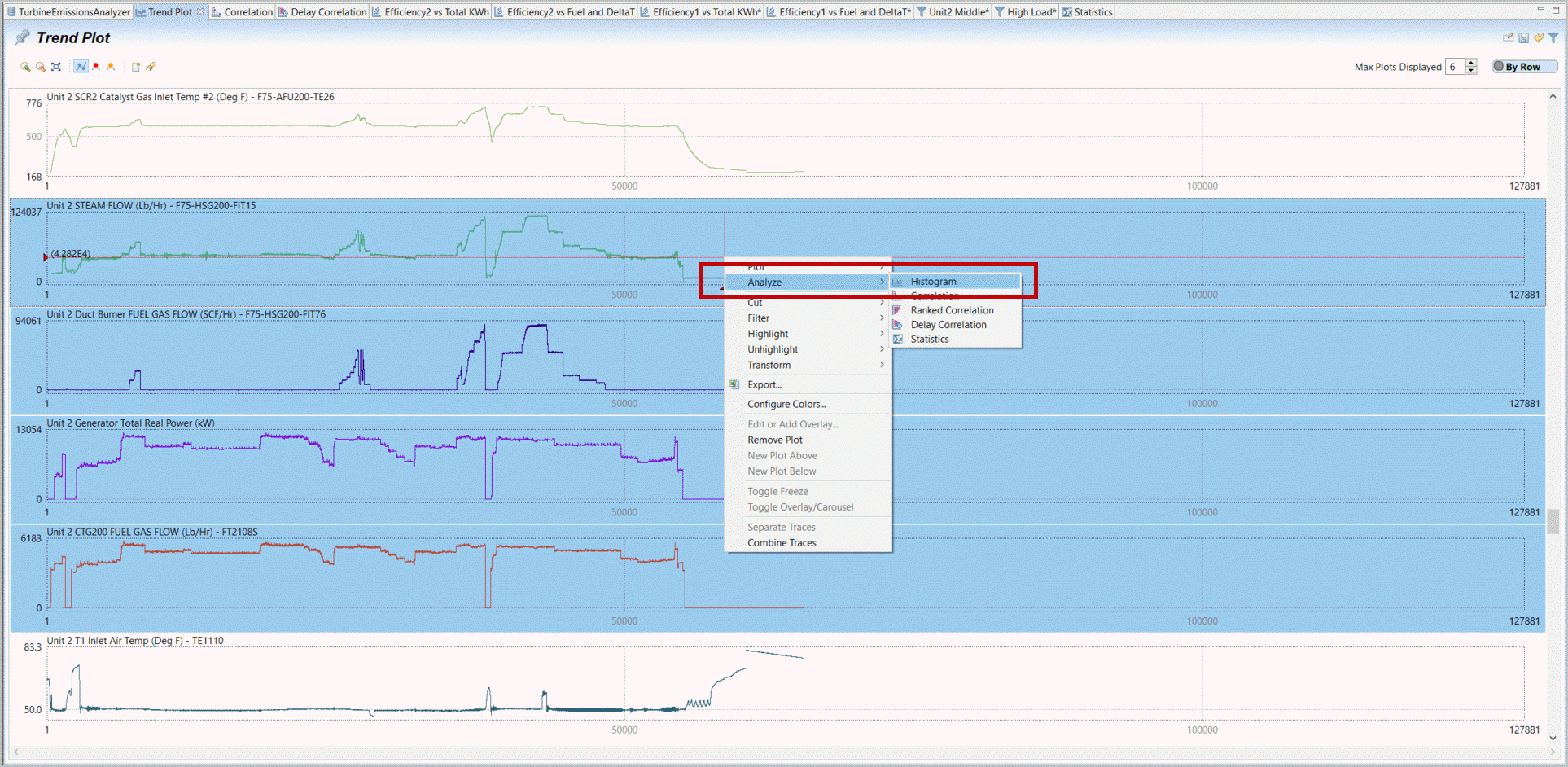
- Selectthe TrendPlot,scrolldown to the Unit 2 Temperatures and Flows andperforma Multi-Select on flows from “Unit 2 Steam Flow” to “Unit 2 CTG200 Fuel Gas Flow”. On any of the selected trends,right mouse-clickandselect“Analyze” and “Histogram”.Select Variables for Histogram Analysis
- Histograms display the range of data, by populations (height of vertical bar) distributed in bins. Select and unselect “Accumulation” that totalizes the bin volumes across the range (e.g. what value is 95% of the values).Histogram of Unit 2 Flows
 Accumulated Histogram
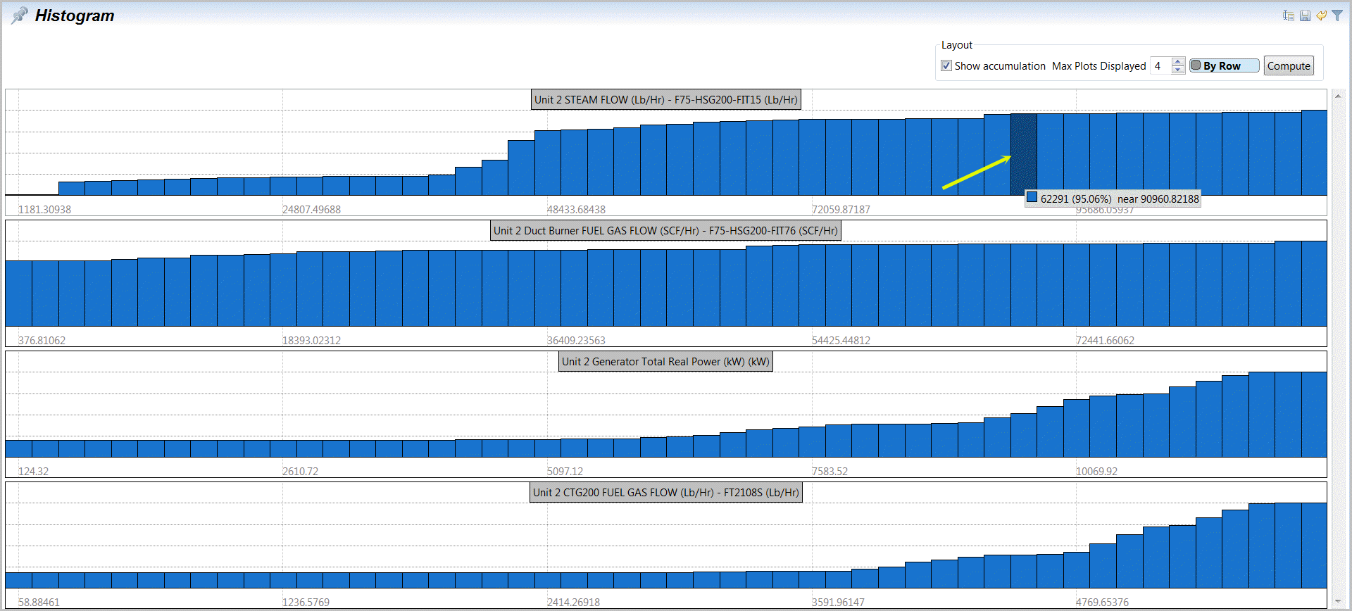
- Select All
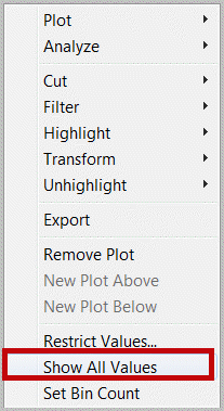
 andRight Mouse-Clickon one of the plots andSelect“Restrict Values”. Note also that there is also an option to “Set Bin Count” if you need more or less resolution.Histogram Plot Options, Select Restrict Values
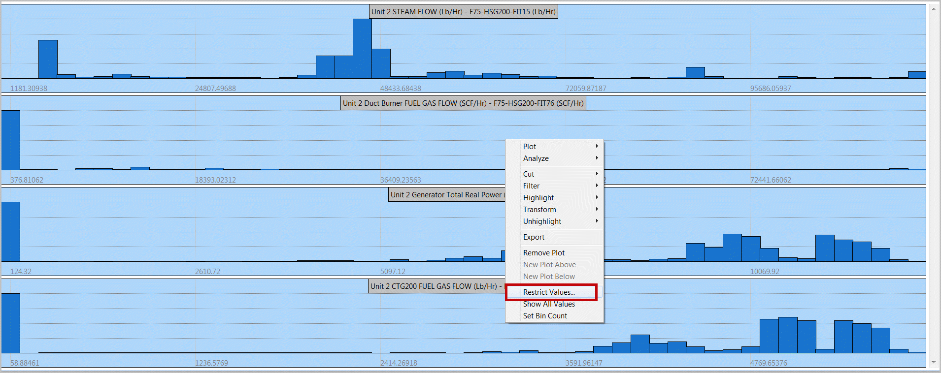
- Occasionally when comparing common values it is useful to display histograms on a common range.Setrange to include the maximum data (Select all four tags and “Use Min/Max from Selection”). Alternativelyset(manually change) the range (Minimum and Maximum Value) from 0 (eliminate below 0 data) and leave 118,130 (which is preset to that overall Max) andselectOK.You may select and range different histograms to different ranges. Select desired tags.Align Ranges and Data Across Histograms
 Histograms Aligned with a common Range
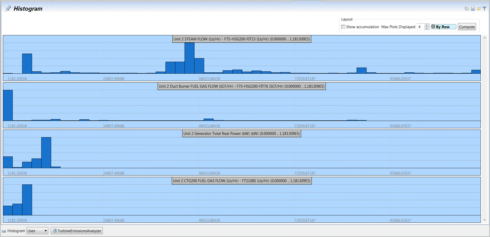
- Undo this range set, with anotherright mouse-clickon the histogram andselecting“Show All Values”.Histogram Plot Options
- Selectthe histogram tab and the filter Icon in the display (on the right histogram header). Add the filters for High and Medium Load. Select OK. You may unselect (i.e. clear) plots with Shift mouse-click.Select Filter on Histogram
 Apply Two Filters on Unit 2 Histogram
 Histogram with two red/blue filters
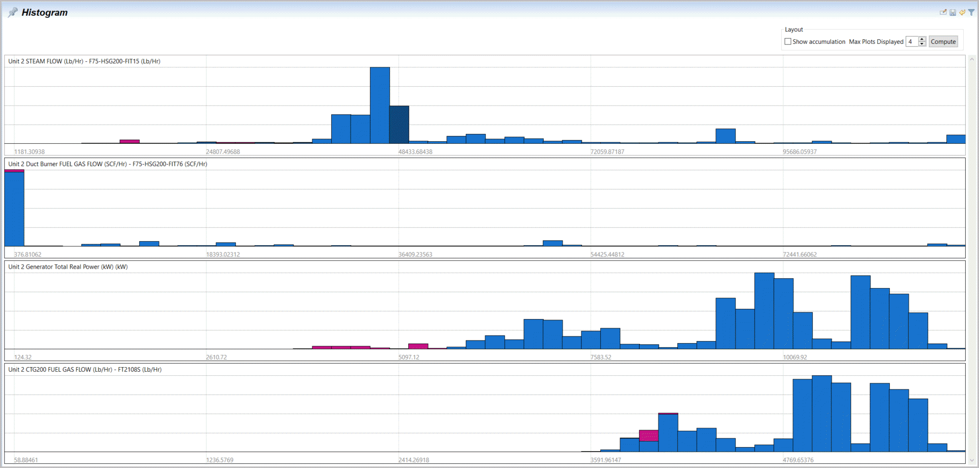
- This may seem like all the data.Selectthe filter icon again andselect“Show Unfiltered Data”.SelectOK.Edit Active Filters from Filter Icon
 Select Show Unfiltered Data
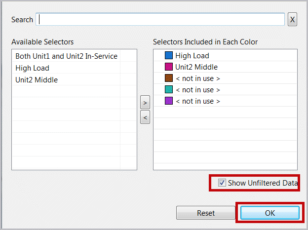
- You will find unfiltered is most of the data but unfiltered in histogram is 'all' data. So the stack is all versus high load and medium load data. Move your cursor over different sections of the vertical stacked bars. Each pattern is shown (not hidden by overlay plots), so check the quantity of patterns represented (the percent is the percent of the section data) and you will see small differences, while most patterns available are either in the selected high or medium times.Histogram with Filtered and Unfiltered Data
 Data presented is number of patterns and data percentage
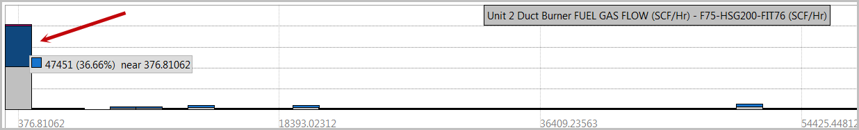
- Selectthe original “Correlation” plot. We will study Unit 2 Inlet NOx.Observewhat appears more or less correlated with Inlet NOx (remember inlet NOx is before the SCR and Exhaust NOx is after SCR which is used to reduce emissions). The larger diagonal is 100% (Inlet NOx versus NOx/itself) and stronger correlations are larger boxes such as Inlet O2 (the first blue box – a negative/reflective correlation of -0.559 (-55.9%).Scrolldown,observethe second column to look for other correlated variables. From the 100% NOx versus O2,right mouse-clickandselect“Analyze” and “Ranked Correlation”.Correlation Plot Investigating Inlet NOx
 Select Ranked Correlation from NOx versus NOx (Same variable).
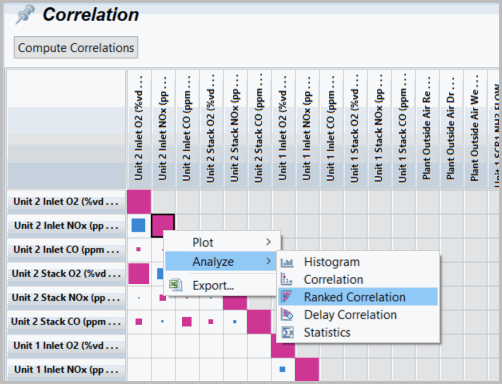
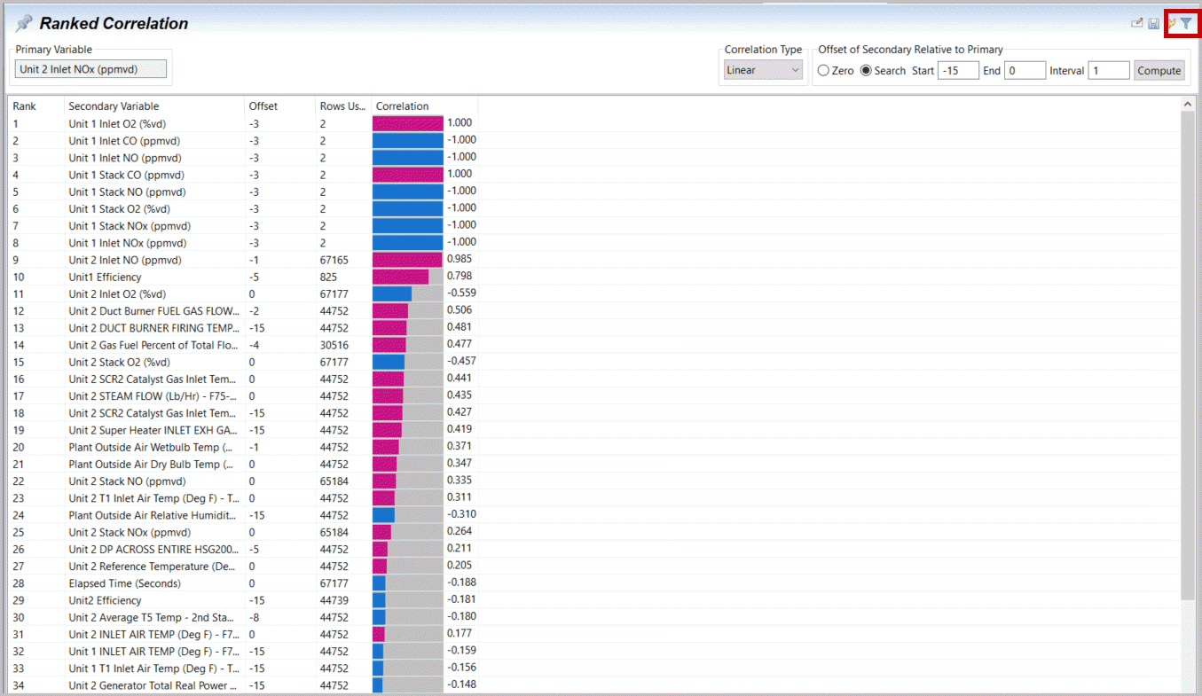
- Unit 1 Efficiency shows a high correlation with Unit 2 NOx (but we know to ignore this, it also indicates there are only 830 common rows used, compared to other results with closer to 50,000 patterns to evaluate). Correlation can be misleading and human consideration is a better way to confirm or discover real information in your data. After Inlet O2, information on the duct burner and pilot manifold appear relevant. To look at a delay search (increasing correlation search areaselectDelay “Search” andenter-15 to 0 at an interval of 1. Thenselect‘Compute’.Ranked Correlation with Unit 2 Inlet NOx
 Select Delay Search Range
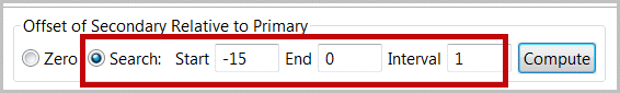
- Correlation increases slightly with the broader search range. Ignore Unit 1 data – in particular those variables with very few rows (i.e. 100% correlated, but only using 2 rows). Only small changes occur here and combustion is a rapid process operation.Ranked Correlation with Delay Search
- Compute again after selecting the “High Load” and “Mid-Load” filters. Results differ measurably after we remove transient and outliers. This is probably a better evaluation.Double-clickboth filters.Double-clickthe selector <All of> to change to “ANY”. Select “Calculate” again.Set Filters for Delay Search
 Ranked Correlation with Filters and Delay Search
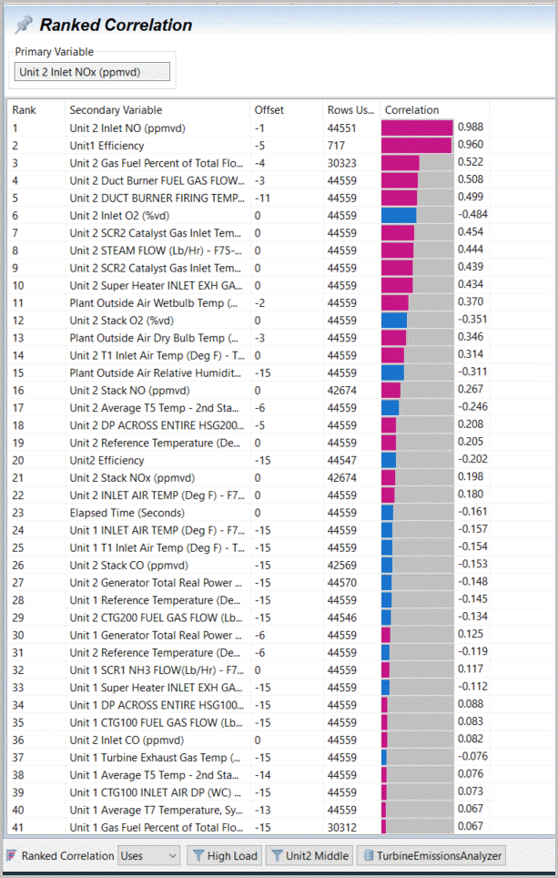
User should then select relevant, high priority features as candidate inputs for modeling NOx.
Multi-select
displayed variables, then right-mouse-click
and select
Export.Ranked Correlation Plot, Select Variables for Export

Provide Feedback