Optional Additional Steps

If you want to understand more features, close all but the first two windows (xy, correlation…). Select
the Trend Plot tab. Selecting
(with ctrl mouse-click) Unit 2 Fuel Gas Flow along with DP across entire HSG and CTG200 Inlet Air DP (below Fuel Gas) and generate
a Delay Correlation between Fuel gas flow (your primary/X variable) and the two pressure drops. (multi-select 3 variables, right mouse-click Analysis, Delay Correlation).

Close tabs by the x-box on each tab label or with Close Tabs to the right

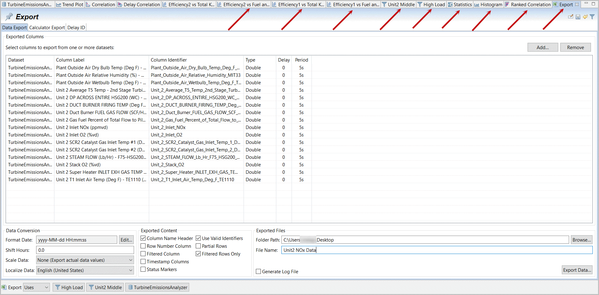Create Delay Correlation between Pressure Drops and Fuel Gas Flow on Unit 2

Select Primary Variable for Delay Correlation plots

Select
Fuel Flow as primary variable.

Change default times to -10, +10 and 1. Note the 5 and 10 second (1 and 2 row) delays.

Delay Correlation with Unit2 Fuel Gas Flow

Select
the original Dataset Summary tab (TurbineEmissionsAnalyzer). Enter
DP in the Search field. This filters our data down to these noisy DP signals. Select
all

Right mouse-click
and select
a Plot, Trend Plot of these DP Variables only.

Select
two Unit 2 DP values (with multi-select right mouse-click
and select
Transform, Smooth data (expave for exponential average smoothing filter).

Create ExpAve Data Filter on Unit 2 DP Variables

ExpAve is the simpler first order data filter. Enter
0.15 for the Value. This makes a filter, Filtered_Measurement[t] = (1 - Value) * Filtered_Measurement[t-1] + Value * New_Measurement[t]. Select
OK.

Select
the two Unit 1 DP cells, right mouse-click
and select
Transform and Dynamic filter (arx). This is a more sophisticated filter reflecting a dynamic response pattern (autoregressive exogenous model if you are looking for party topics).

Change
the Model Type from Zero Order (delay shift) to First order. Enter
(we need to include time units with each time value):

Time Interval 5s

Delay 0s

Gain 1

Time Constant 25s

Lead Time 0s

Select
OK.

NOTE:

Note
that a zero order model allows you simply to shift columns by any number of rows (e.g. align correlated patterns into a single row so that you could shift Fuel Gas flow shown in step 71 by one or two 5 second rows and match on a common row (for steady-state machine learning as mostly assumed).

Enter Configuration for Dynamic Filtering

Both sets of Unit’s DP measurements are now filtered.

Confirm this has impacted results by selecting
the “Compute” button on the Delay Correlation plot.

Increasing Delays with Filtering on DP data

Select
the “Trend Plot” and the scroll bar one variable down so that “Unit 2 Inlet NOx” is at the top of the plots. Right mouse-click
on “Unit 2 Inlet NOx” and select
“Toggle Freeze”.

Zoom in
(by dragging across a range) to observe an interesting, active region of Inlet NOx movement.

Then scroll down
to various Unit 2 parameters to observe if visually dramatic spikes in NOx appear related to particular process changes. Did you notice the shape similarity between NOx and duct burner fuel gas flow? Also spikes in NOx related to drops in T5 Temperature (and further down even more Fuel gas percent of total flow to pilot manifold). Sometimes just observing your data can be very enlightening.

Compare Data with Frozen Target NOx with Zoom

Select
the most interesting of these (NOx, plus Steam Flow, plus Duct Burner Fuel gas Flow, plus T5 Temperature and Percent of fuel to pilot manifold – right mouse-click and select a “Carousel Plot”. Select
“Unit 2 Inlet NOx” as Top Row (this may be at the bottom of the list).

As with Toggle Freeze, NOx is not frozen, but you may scroll from one to another of the variables by putting your cursor on the second (not primary) plot and a right or left arrow is available to jump through your variable list.

You have explored the major features of Data Explorer. Now take your own data for a spin.