Performing a Time Merge
To time merge data:
- Do one of the following:
- Select the manifest and click [Time Merge].
- Go toDataseticon > Time Merge. You will be asked to select a dataset.
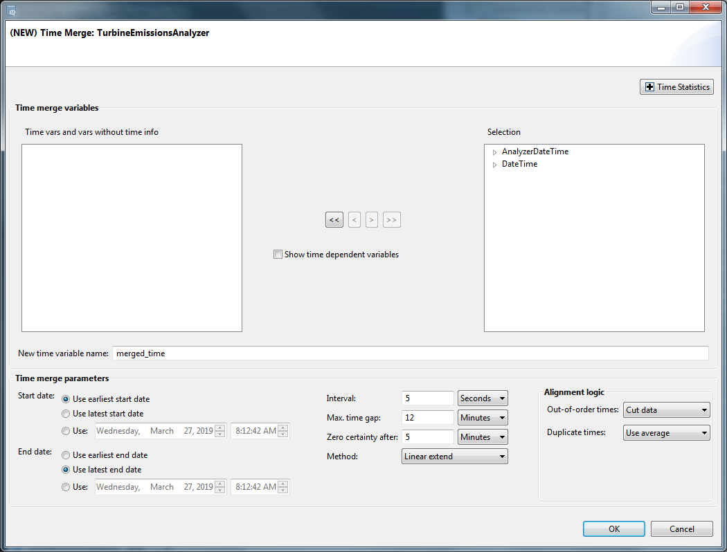
TheTimeMergedialog displays.Time Merge Dialog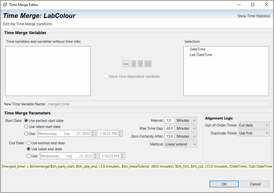
- In the main dialog, select the time variables you want to merge (AnalyzerDateTime and DateTime in the above image) and add them to the Selection box using the right arrow keys.TheShow time dependentvariables checkbox changes the display so that, in addition to the date/times and unattached variables, it shows the other variables that reference each date/time. These variables are always affected by a time merge of their date/time reference, regardless of whether they are displayed. Time merge calculations are applied directly to raw and independent variables; computed variables inherit the effect of the time merge on the variables from which they are computed.
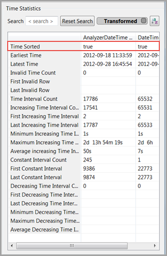
- Click [Show Time Statistics] if you want to review statistics relevant to the time merge. For example, you may need the information to decide on an appropriate time interval for the merge, or you may want to see the start/end times for the existing time variables.Time Statistics
- Define the following and click [OK].
- Start/End Date: Define the date from which the merge will start and end.The range of the time merge can be set to the Earliest Start and Latest End or the Latest Start and Earliest End of all date/time columns in the dataset at the time the time merge is executed. You can override these choices and fill in a specific starting and ending date and time, but those values will be retained in the dataset's transform list and will prevent the use of any data outside that range.
- Interval: Define the time difference between successive rows in the resulting time column. Enter in the amount and select its units from the option list.
- Max. time gap: Enter in the amount and select its units from the option list. If you will be using this dataset to model a process, the maximum time gap should be set to a value greater than the time merge interval but less than the time frame over which extrapolation or interpolation would introduce significant errors. This maximum time gap is therefore a function of the speed of the process as well as the time merge interval.The maximum time gap is an optional value used to control whether a gap in the data (before the merge) is filled by the time merge or is left blank. If a gap in the data is smaller than the specified maximum time gap, the time merge expands data to fill the gap. If a gap in the data is larger than the maximum time gap, the time merge indicates the gap by a data point with a Blank status. If all columns are filled with multiple rows of blanks, time merge collapses them into a single row of points with a Break status.Breaks in a dataset are used to set a boundary between groups of data that are so far apart in time that you cannot sensibly interpolate between them. Breaks are used to prevent the product from finding any spurious time-dependent relationship between them when it trains a model or analyzes time-delayed data. Therefore, a Break is completely different from any other type of “bad” data. All transforms that operate on multiple rows of data treat Break as a boundary, not as a single bad data point. If you are using only user-specified models, the dataset values do not matter (except that the range of the data is used to set default variable bounds and constraints).
- Zero certainty after: Define the distance from known data that causes a certainty of zero (i.e., MaxCert). Enter the amount and select its units from the option list.Time merges may generate new data by extrapolation or interpolation. For each point, a record is kept of whether it existed before the time merge or whether it was generated, and, if generated, how far away it was from known data; this record is called certainty.Certainty values are generated by the $TimeMerge transform and do not use any other information about the variable. If you time merge the same variable twice, its certainties after the second time merge do not consider any poor certainties it may have had resulting from the first-time merge. If you will be making use of certainty information, avoid time merge the same variable more than once.
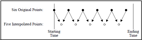
- Method: Select one of the following time merge methods (Boxcar, Linear Extend, Spline Extend, Linear, or Spline).Boxcar simply repeats the most recent value while Linear and Spline interpolate. Keep in mind that interpolation can cause one or more data values to be lost at the endpoint:Interpolated Points
 For interpolated points, the LinearExtend and SplineExtend options function the same as ordinary Linear and Spline, but they also they repeat the last original value until the specified ending time is reached:Extend Interpolated Points
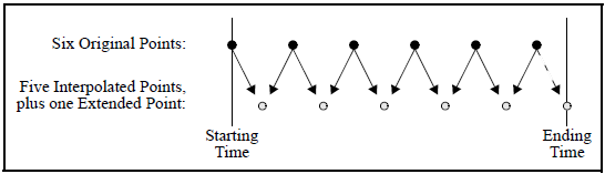 NOTE:Boxcar extrapolation estimates intermediate values by projecting from past values, but Linear and Spline interpolation estimates intermediate values using both past and future values. Be careful that your model does not rely on future values of inputs that will not be available when the model is used with current, rather than historic, data. Compensate by time-lagging interpolated inputs.Spline interpolation over relatively large gaps tends to produce spikes in the resulting values. If gaps in the data are large, you may get better results by doing a Linear time merge first, followed by a Spline.
 - Out-of-order times: time merge calculations can only be applied to date/time values in strictly increasing order. Check “Decreasing Time Interval Count” in Time Statistics to confirm the need for this option. The two option lists are used to specify how to handle values out of order:
- Cut Datathrows out any data that is in decreasing time order.
- Sort Datasorts the entire dataset while making the time merge calculations.
TIP:If the time values are in random order, sorting can be extremely slow. It may be preferable to sort the dataset first (using a series of $sort transforms), export the sorted data to a CSV file, and create a new dataset that is already sorted. - Duplicate times: : if the dataset includes any duplicate times, define how duplicates will be handled. Check “Constant Interval Count” in Time Statistics to confirm the need for this option.
- Use Firstuses the data at the first occurrence of the time and ignores all repetitions of the time.
- Use Lastuses the data at the last occurrence and ignores any earlier reports.
- Use Averagesaves all values (per variable) at duplicate times and averages them.
When the time merge begins, a $TimeMerge transform is generated and applied to the dataset. This transform may force some other transforms already on the dataset to be re-evaluated.
For example, using the data defined in the sample figures, a time merge could be configured as follows:
- Time Sorted indicatestrue(see Figure: Time Statistics), so leave Out-of-order times as is (Cut data).
- The time statistics around intervals may be complex and can obscure our intervals for merged time. Knowing that original data capture is every 5 seconds for process data and every 30 seconds (in the tutorial) for Emissions analyzer data, set the following:
- Interval: 5 seconds (on other cases, you could choose 30 seconds or a different frequency). We generally want all available data and include capabilities to evaluate time relationships.
- Max.time gap: 12 minutes. We generally want to maintain all useful intervals but avoid interpolating between dynamically independent stationary conditions (i.e. maximum time to steady state of system of focus).
- Zerocertaintyafter: 5 minutes. We generally want to zero certainty after the predominant time to steady state (less conservative than Max Time gap).
- Method: Linear Extend (This defines the zero interpolated value certainty after and interpolation method.)
- Duplicate times: Use Average (Use this setting when there are multiple constant intervals.)Time Merge Configuration
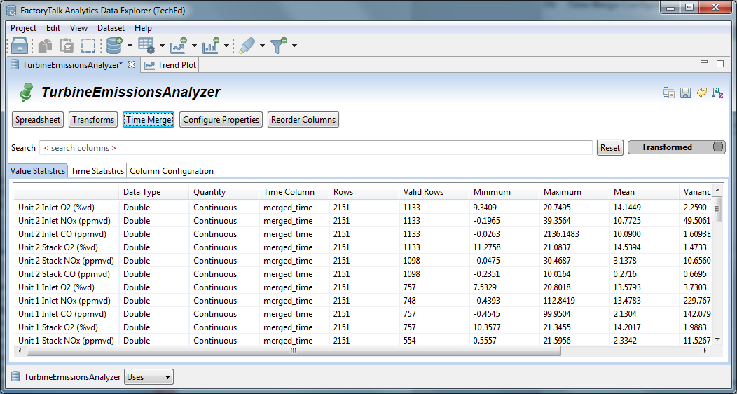
After the time merge is complete, the data is now on a common time basis so that any analysis or machine learning that assumes a time alignment between different sources can use the data. The Time Column reflects the merge.
Time Merge Completion
Provide Feedback